Lineweaver–Burk Plot with Example

Spread the love

Lineweaver–Burk Plot

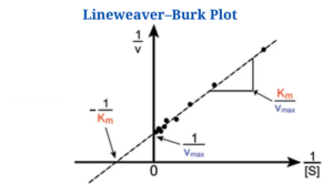
The Lineweaver–Burk plot (also known as the double reciprocal plot) is a graphical representation of enzyme kinetics used to determine the Michaelis-Menten parameters $V_{ma x}$ (maximum reaction velocity) and $K_{m}$ (Michaelis constant).

Because V_max is attained at endless substrate concentration, estimating Vmax and thus Km from a hyperbolic plot is impossible.
Due to this issue, Lineweaver and Burk modified the Michaelis–Menten equation into a straight line equation.
The Lineweaver–Burk plot (also known as the double reciprocal plot) is a pictorial depiction of the Lineweaver–Burk equation of enzyme kinetics, which was presented by Hans Lineweaver and Dean Burk in 1934.
This figure is derived from the Michaelis–Menten equation and is denoted as follows:

where V represents the reaction velocity (reaction rate), Km denotes the Michaelis–Menten constant, V_max denotes the maximum reaction velocity, and [S] denotes the substrate concentration.

It produces a straight line with a y-axis intercept of 1/V_max and an x-axis intercept of K_m/V_max. The slope of the line is equal to K_m/V_max.
V_maxand K_m can be calculated experimentally by measuring V₀ at various substrate concentrations. Then, for 1/V₀ vs 1/[S], a double reciprocal or Lineweaver–Burk plot is generated.

A Lineweaver–Burk plot can be used to discriminate between competitive and noncompetitive reversible enzyme inhibitors.
It is an effective method for determining how an inhibitor interacts to an enzyme.
If V0 is measured at multiple substrate concentrations in the presence of a fixed dose of inhibitor, a Lineweaver–Burk plot can be used to detect competitive inhibition.
On the Lineweaver–Burk plot, a competitive inhibitor increases the slope of the line and changes the intercept on the x-axis (because K_m is increased), but leaves the intercept on the y-axis unaltered (since V_max remains constant).
Noncompetitive inhibition can also be identified on a Lineweaver–Burk plot because it raises the slope of the experimental line and changes the intercept on the y-axis (due to a drop in V_max), but leaves the intercept on the x-axis unaltered (since K_m remains constant).

Advantages:

Linearizes the Michaelis-Menten equation for easier analysis.
Allows clear determination of $V_{ma x}$ and $K_{m}$ .

Disadvantages:

Can amplify errors at low substrate concentrations (since reciprocal transformation exaggerates small values).
Other plots (e.g., Eadie-Hofstee) may be better for certain datasets.

Uses of Lineweaver–Burk Plot

Identifying enzyme inhibition types:
- Competitive inhibition: Alters $K_{m}$ but not $V_{ma x}$ .
- Non-competitive inhibition: Alters $V_{ma x}$ but not $K_{m}$ .
- Uncompetitive inhibition: Alters both $K_{m}$ and $V_{ma x}$ .

Lineweaver-Burk Plot Worked Example

Experimental data for an enzyme-catalyzed reaction:

[S] (mM)	v (μM/min)
1.0	12.0
2.0	20.0
4.0	30.0
8.0	40.0
10.0	44.0

Step 1: Calculate 1/[S] and 1/v

[S] (mM)	v (μM/min)	1/[S] (mM⁻¹)	1/v (min/μM)
1.0	12.0	1.0	0.083
2.0	20.0	0.5	0.050
4.0	30.0	0.25	0.033
8.0	40.0	0.125	0.025
10.0	44.0	0.1	0.023

Step 2: Plot Interpretation

The Lineweaver-Burk plot shows a straight line where:

Y-intercept = 1/V_max
Slope = K_m/V_max
X-intercept = -1/K_m

Step 3: Determine V_max and K_m

1. Find V_max from Y-intercept:
Experimental y-intercept ≈ 0.02 min/μM
1/V_max = 0.02 → V_max = 1/0.02 = 50 μM/min

2. Find K_m using slope:
Experimental slope ≈ 0.06 min
Slope = K_m/V_max → K_m = Slope × V_max = 0.06 × 50 = 3.0 mM

Alternative method using x-intercept:
Experimental x-intercept ≈ -0.33 mM⁻¹
-1/K_m = -0.33 → K_m = 1/0.33 ≈ 3.0 mM

Final Results

V_max = 50 μM/min
K_m = 3.0 mM

Conclusion

The enzyme has a maximum velocity of 50 μM/min and a Michaelis constant (K_m) of 3.0 mM, meaning it reaches half-maximal velocity at 3 mM substrate concentration.

Lineweaver–Burk Plot Citations

David Hames and Nigel Hooper (2005). Biochemistry. Third ed. Taylor & Francis Group: New York.
Smith, C. M., Marks, A. D., Lieberman, M. A., Marks, D. B., & Marks, D. B. (2005). Marks’ basic medical biochemistry: A clinical approach. Philadelphia: Lippincott Williams & Wilkins.
https://en.wikipedia.org/wiki/Lineweaver%E2%80%93Burk_plot

Related Posts